Cosmo4D

Large Scale Structures in the Universe

In physical cosmology, structure formation refers to the formation of galaxies, galaxy clusters and larger structures from small early density fluctuations. The universe, as is now known from observations of the cosmic microwave background radiation, began in a hot, dense, nearly uniform state approximately 13.8 billion years ago. However, looking in the sky today, we see structures on all scales, from stars and planets to galaxies and, on still larger scales still, galaxy clusters and sheet-like structures of galaxies separated by enormous voids containing few galaxies. Structure formation attempts to model how these structures formed by gravitational instability of small early density ripples.

Below is a video (by Yu Feng) that demonstrates this process. Structures (filaments and halos) form as time evolves. At the center of halos where the density is highest, galaxies and super-massive black holes form and emit light that we can observe with telescopes.

• Further Readings (Wikipedia)

Theory of structure formation

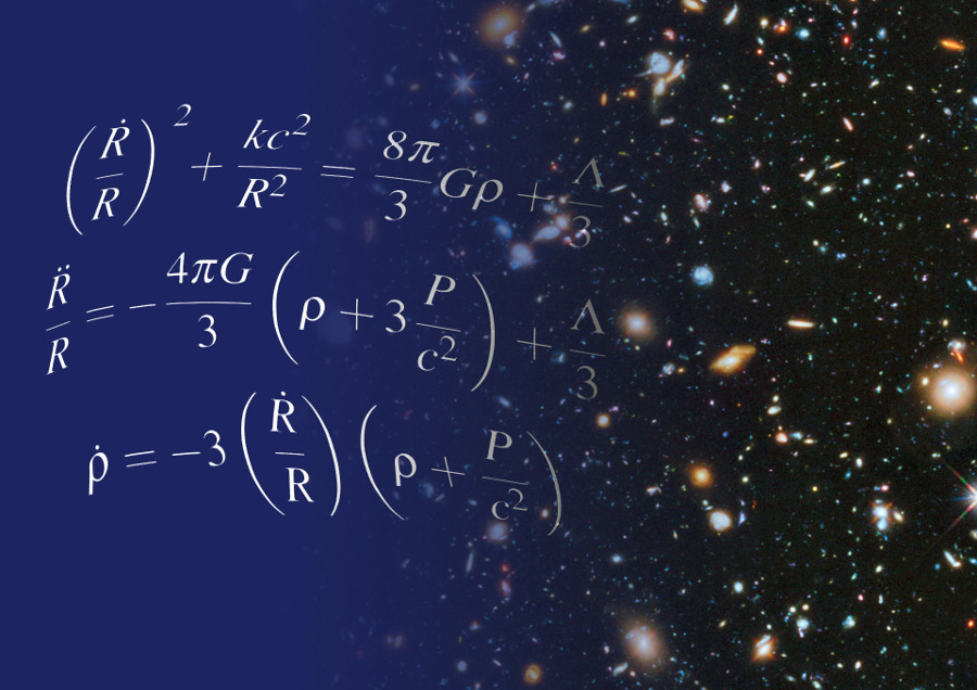
We do have a relatively accurate understanding of the physical theory behind the Universe.

The standard model of cosmology, \(\Lambda\)CDM model, was discovered around the 1990s, and the current observational data strongly supports this model.

The model describes the Universe with 6 parameters:
• mass fraction of cold dark matter \(\Omega_C \sim 0.260\),
• mass fraction of baryons \(\Omega_b \sim 0.049\),
• hubble constant \(H_0 \sim 67.7 \mathrm{km s^{-1} Mpc^{-1}}\),
• amplitude of primodial fluctuation \(A_s = 2.44\times 10^{-1}\),
• reionization optical depth \(\tau = 0.07\),
• primodial spectrum index \(n_s = 0.967\).

Current and next generation observations are constraining these parameters to sub-percent level accuracy. Extensions to the model includes a varying dark matter equation of state, non-gaussianity of the primodial fluctuation, gravity beyond generalitivity, and tensor modes in the primodial fluctation.

The gravitional effect of dark energy drives the expansion of the universe. On this expanding background, the matter component (dark matter and baryon) collapses by gravity to form structures, halos. Galaxies form in the center of halos, emitting light for us to observe. The effect of baryons are secondary, consisting of hydrodynamics, radiation, atomic cooling, and feedback from stars and blackholes.

Advanced large scale parallel computer algorithms, most notably N-body simulations provides fast and accurate predictions of the primary gravitional component of structure formation. Our current theoretical understanding of structure formation can accurately predict the formation of large scale structure for any given initial condition and cosmological parameters. The level of systematics in the model is subdominant comparing to the level of uncertainties from observations.

• Further Reading (Review by Joel R. Primack)

Power and limitation of data

Observational data has been the most intrumental tool for us to understand our Universe. Observational data sets are growing in size. Our current way of comprehending the observed data set is by model fitting / sampling over the 2 point statistics of observed data. The existing approach has been extremely succesful. For example, The following figure shows the best fit model of the cosmic microwave background power spectrum against data measured from the Planck satellite. The uncertainty in data is very small, and the agreement between model and data is very high.

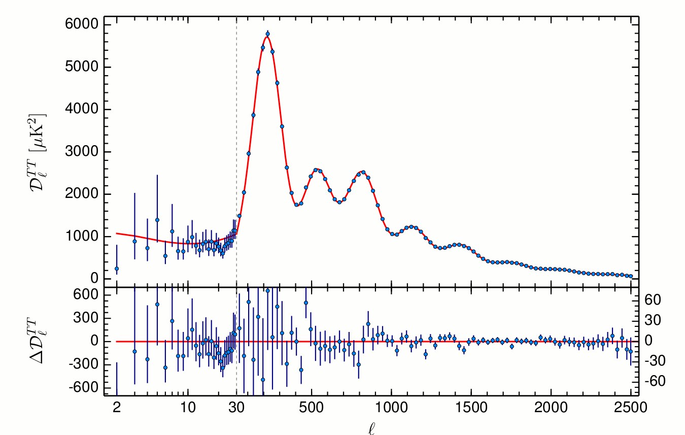
With this approach, however, it is hard to quantify the amount of information that has been fully recovered from the data. The data that goes into the fitting is heavily compressed into 2 point statistics, a 1 dimentional function. We do expect the loss of information due to this compression.

In addition, because the speed of light is finite and the universe is vast, when we observe the universe, we only see it at the time light is emitted from a distant past. The following figure shows how the age of the observed universe increases as the distance to us increases.

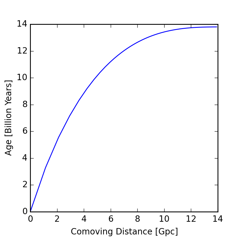
As an example, the Planck and WMAP satellites observed the cosmic microwave background radiation in the universe at a distance of 14 Giga-parsec (45.5 billion light years) away, and at a time of 13.7 billion years ago. The light appears to be travelling faster because light travels as the universe expands, an effect due to General Relativity. As another example, one of the main sample of galaxies observed by the Sloan Digital Sky Survey, the CMASS sample, was a population of galaxies 2 Giga-parsec (6.76 billion light years) away, and at a time of 5.44 billion years ago.

It is also slightly messy to directly include the difference of structure at different distance in the model.

With Cosmo4D, we take a cleaner approach. We will define the model \( S \) at the time of the initial density flucutation in the Universe. A forward modelling dynamics \( F(S) \) relates the initial condition to the observed universe, where we define the goodness of the model with a plain \(\chi^2 \sim (F(S) - F(D))^2 \). The full model includes 3 spatial dimensions and the evolution in time. Hence \[ 3 + 1 = 4, \] Cosmo4D is phyiscal cosmology in the lingo of machine learning.

We are actively developing the method. In this demo, we will show two examples:

• Reconstruction of Density from Cosmic Shear (2-D spatial + 1-D time + Linear dynamics)
• Reconstruction of Dark Matter Initial Condition (3-D spatial + 1-D time + Non-Linear dynamics)

But first, let's take a look at the L-BFGS optimization algorithm that formed the backbone of Cosmo4D.

• Next

L-BFGS

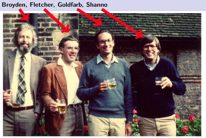
The BFGS (Broyden, Fletcher, Goldfarb, Shanno) algorithm is a quasi-Newton algorithm for nonlinear optimization. By using the previous iterations it calculates an approximation to the inverse Hessian matrix. However, storing the state vector of all of the previous iterations can require a lot of memory (Keep in mind, decribing the inital condition of the universe requires millions or billions of dimensions). L-BFGS stands for "Limited memory BFGS" which stores only the state vector of last few iterations, but is mathematically shown to work almost as well as storing all of them.

To illustrate the algorithm, we borrow this image form Wolfram Research, which shows the iterations of L-BFGS. We see that after each iteration the state vector is always moved towards a local minima of the cost function. The direction of the motion is closely related to the derivative of the cost function.

• Further Reading (Aria's Blog)

Initial simulation

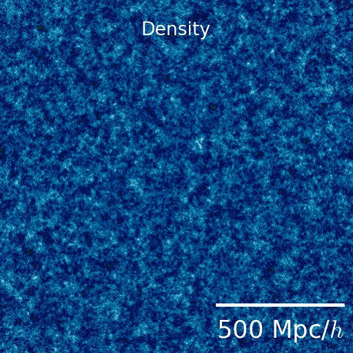
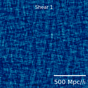
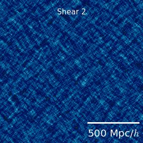
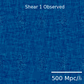
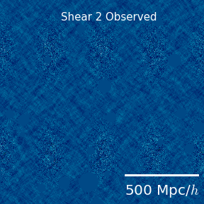
The initial density field is simulated from a given power spectrum. What we observe through weak lensing is not the density field directly, but rather two shear fields. Shear 1 describes distortions in the horizontal and vertical directions, and shear two describes distortions in the diagonal directions.

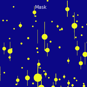
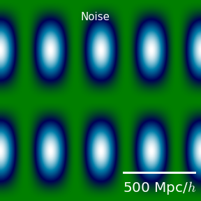
Mask and noise

Parts of the sky are unobservable because of bright stars. Also, our observations are noisy. Here we show the mask and the noise. The yellow parts in the mask are parts of the sky where we don't have data because of a bright star. The noise level in this simulations varies across the sky as shown in the image below (the white parts have the largest amount of noise, whereas the green parts are the least noisy).

Observed shear (with mask and noise)

The images below show the actual observed shear, including the noise. As we can see, in some parts the noise level is higher, which results in a more blurry image. Also, after adding noise we can still see the structure on the largest scales more or less clearly, but the small scale structure is completely washed out by noise.

Reconstructing the initial density field

The video below (left) shows the iterations of the L-BFGS algorithm trying to find the best-fit initial density field. The image in the middle shows the original density field, and the image on the right shows the final reconstruction.

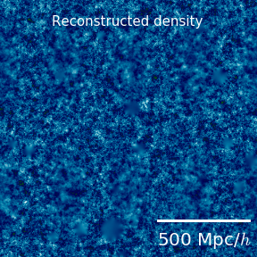
We can see that the reconstructed field matches the original field very well. However, the match is not as good in the regions with high amount of noise and the masked regions, as expected.

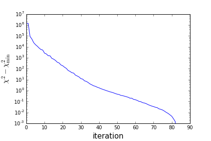
L-BFGS convergence

Power spectrum deficit

As we can see above the reconstructed density field matches the initial simulation very well. However, we can see that the structure on very small scales is missing in the reconstruction. That is because of noise. We can see the loss of power on small scales in the following plot of the power spectrum, i.e. the two-point function.

\(<\delta(\mathbf{k})\delta(\mathbf{k^\prime})>=P(k)\delta_{\mathbf{kk^\prime}}\)

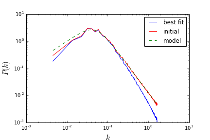
The green curve shows the original model from which the initial density field is simulated. The power of the simulated field is shown in red, and the power of the reconstructed field is shown in blue. As we can see, there is deficit of power for large \(k\), i.e. small scales. There is also loss of power for the largest scale (smallest \(k\)). This is because the weak lensing data is insensitive to the mean density field, so the reconstructed field will have zero mean.

Power spectrum reconstruction

We reconstruct the missing power in two steps. First, we perform a few simulations of just noise and run the same optimization algorithm. This allows us to estimate the noise bias, i.e. how much of the reconstructed power comes from noise. Next, we perform simulations of the data, but we inject a small amount of extra power in one of the bins. We then run the same optimization method again. The reconstructed density field will have some extra power in some of the bins. This allows us to estimate the response of all the bins to a small change of initial power in a given bin. By repeating this step for all the bins we are able to reconstruct the full Fisher matrix. Using the Fisher matrix and the noise bias we can then get an estimate of the original power spectrum, including error bars.

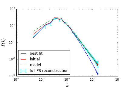
The plot above shows the reconstructed power spectrum with the error bars in cyan. The agreement with the original model power spectrum (in green) is very good.

Definitions

Let's define a few metrics. These are shown in the video.

The cost function (smaller is better)

\[ \chi^2 = \sum \frac{(F(S) - F(D))^2}{\sigma^2} \]

Cross correlation coefficient (closer to 1 means higher correlation)

\[ X[A, B] = \frac{P_{A, B}}{\sqrt{P_{A} P_{B}}}. \]

Power spectrum recovery ratio (closer to 1 means better recovery)

\[ R[A, B] = \frac{P_{A}}{P_{B}}. \]

L-BFGS iterations successfully reduce \( \chi^2 \). This can be visually seen as the model converges. to the data. Very quickly (with < 100 iterations), the model already agrees with the data at large scale (small k).

The initial condition is recovered, but the a bias at intermediate scales, indicating we need to use the power spectrum recovery method in the cosmic shear example to unbias the power spectrum estimator. The residual has very low power, though slightly correlated with the data, an indicator of possible over-fitting. This is a topic that we are currently investigating.

Four panels are:

• top left : Projection of the model at present day \( F(S) \)
• top right : Projection of the model at initial condition \( S \)
• bottom left : Variance of residual at present day \(\mathrm{VAR}(F(S) - F(D)) \)
• bottom right : Variance of resitual at intial condition \(\mathrm{VAR}(S - D) \)

Insets are :

• top : \( \chi^2 \) as a function of L-BFGS iteration.
• bottom left : at present day,
  Red Solid : \( X[F(S), F(D)] \)
  Blue Solid : \( R[F(S), F(D)] \)
  Red Dotted: \( X[F(S) - F(D), F(D)] \)
  Blue Dotted: \( R[F(S) - F(D), F(D)] \)
  
• bottom right: at inital condition,
  Red Solid : \( X[S, D] \)
  Blue Solid : \( R[S, D] \)
  Red Dotted: \( X[S - D, D] \)
  Blue Dotted: \( R[S - D, D] \)